Speech2Face

This repository has all the codes of my implementation of Speech to face.

Requirements

Python 3.5 or above
Keras
TensorFlow
Librosa
keras_vggface
opencv
Dlib

How much can we infer about a person’s looks from the way they speak? In this paper, we study the task of reconstructing a facial image of a person from a short audio recording of that person speaking. We design and train a deep neural network to perform this task using millions of natural Internet/YouTube videos of people speaking. During training, our model learns voice-face correlations that allow it to produce images that capture various physical attributes of the speakers such as age, gender and ethnicity. This is done in a self-supervised manner, by utilizing the natural co-occurrence of faces and speech in Internet videos, without the need to model attributes explicitly. We evaluate and numerically quantify how—and in what manner—our Speech2Face reconstructions, obtained directly from audio, resemble the true face images of the speakers

I have Implemented it in both Pytorch and tensorflow.

The dataset used in this project is Voxceleb1 VoxCeleb is an audio-visual dataset consisting of short clips of human speech, extracted from interview videos uploaded to YouTube. The dataset consists of two versions, VoxCeleb1 and VoxCeleb2. Each version has it’s own train/test split. For each we provide YouTube URLs, face detections and tracks, audio files, cropped face videos and speaker meta-data. There is no overlap between the two versions.

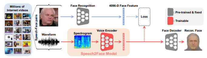Our Speech2Face pipeline, consist of two main components: 1) a voice encoder, which takes a complex spectrogram of speech as input,and predicts a low-dimensional face feature that would correspond to the associated face; and 2) a face decoder, which takes as input the face feature and produces an image of the face in a canonical form (frontal-facing and with neutral expression). During training, the face decoder is fixed, and we train only the voice encoder that predicts the face feature. The voice encoder is a model we designed and trained, while we used a face decoder model proposed by Cole et al. We now describe both models in detail.

Preprocessing

First audio processing,We use up to 6 seconds of audio taken extracted from youtube. If the audio clip is shorter than 6 seconds, we repeat the audio such that it becomes at least 6-seconds long. The audio waveform is resampled at 16 kHz and only a single channel is used. Spectrograms are computed by taking STFT with a Hann window of 25 mm, the hop length of 10 ms, and 512 FFT frequency bands. Each complex spectrogram S subsequently goes through the power-law compression, resulting sgn(S)|S|0.3 for real and imaginary independently, where sgn(·) denotes the signum.

wav_file , sr = librosa.load(path,sr = 16000, duration = 5.98 ,mono = True) ## Reading wav file
stft_ = librosa.core.stft(wav_file, n_fft = 512, hop_length = int(np.ceil(0.01 * sr)),win_length = int(np.ceil(0.025 * sr)) ,window='hann', center=True,pad_mode='reflect') # Getting STFT
stft = self.adjust(stft_) # Making speech 6 sec long.
X =  np.dstack((stft[:,:].real, stft[:,:].imag)) # CONVERING IN CHANNELS
X = np.sign(X) * ( np.abs(X) ** 0.3 ) # COMPRESION

We run the CNN-based face detector from Dlib , crop the face regions from the frames, and resize them to 224 × 224 pixels .The VGG-Face features are computed from the resized face images. The computed spectrogram and VGG-Face feature of each segment are collected and used for training.

img = face_recognition.load_image_file(path)
faceLocation = face_recognition.face_locations(img)[count]
x,y1,x1,y = faceLocation
img = img[x:x1,y:y1,:]
landmark = face_recognition.face_landmarks(img)
for i in list(landmark[0].keys()):
    resultant += landmark[0][i]
landmark = np.ravel(np.array(resultant))
img = cv2.resize(img, (224,224), interpolation = cv2.INTER_AREA).astype('float')
img /= 255.0
return  self.vgg_features.predict(img.reshape(1,224,224,3))`

Face Encoder Model

Our voice encoder module is a convolutional neural network that turns the spectrogram of a short input speech into a pseudo face feature, which is subsequently fed into the face decoder to reconstruct the face image (Fig. 2). The architecture of the voice encoder is summarized in Table 1. The blocks of a convolution layer, ReLU,and batch normalization [23] alternate with max-pooling layers, which pool along only the temporal dimension of the spectrograms, while leaving the frequency information carried over. This is intended to preserve more of the vocal characteristics, since they are better contained in the frequency content, whereas linguistic information usually spans longer time duration . At the end of these blocks, we apply average pooling along the temporal dimension. This allows us to efficiently aggregate information over time and makes the model applicable to input speech of varying duration. The pooled features are then fed into two fully-connected layers to produce a 4096-D face feature.

Loss in Encoder

A natural choice for the loss function would be the L1 distance between the features: kvf − vsk1. However, we found that the training undergoes slow and unstable progression with this loss alone. To stabilize the training, we introduce additional loss terms. Specifically, we additionally penalize the difference in the activationof the last layer of the face encoder, fVGG : R4096 → R2622,i.e., fc8 of VGG-Face, and that of the first layer of the face decoder, fdec : R 4096→R 1000, which are pre-trained and fixed during training the voice encoder. We feed both our predictions and the ground truth face features to these layers to calculate the losses.

def absv(self, a, b):
        return self.__lambda1__ * torch.abs((a/torch.abs(a)) - (b/torch.abs(b))).pow(2)


def PI(self, a, i):
    n = torch.exp(a[i] / self.__T__  )
    d = torch.sum(  torch.exp(a / self.__T__), dim=1)
    return n / d


def Ldistill(self, a, b):
    res = 0.0
    for i in range(a.size[0]):
        res = torch.add(res , self.PI(a, i) * torch.log(self.PI(b,i)))
    return self.__lambda2__ * res`

Face Decoder

It is based on coles Method.We could have mapped from F to an output image directly using a deep network. This would need to simultaneously model variation in the geometry and textures of faces. As with Lanitis et al. [7], we have found it substantially more effective to separately generate landmarks L and textures T and render the final result using warping. We generate L using a shallow multi-layer perceptron with ReLU non-linearities applied to F. To generate the texture images, we use a deep CNN. We first use a fullyconnected layer to map from F to 14 × 14 × 256 localized features. Then, we use a set of stacked transposed convolutions [28], separated by ReLUs, with a kernel width of 5 and stride of 2 to upsample to 224 × 224 × 32 localized features. The number of channels after the i th transposed convolution is max(256/2 i , 32). Finally, we apply a 1 × 1 convolution to yield 224 × 224 × 3 RGB values. Because we are generating registered texture images, it is not unreasonable to use a fully-connected network, rather than a deep CNN. This maps from F to 224 × 224 × 3 pixel values directly using a linear transformation. Despite the spatial tiling of the CNN, these models have roughly the same number of parameters. We contrast the outputs of these approaches.

L1 = self.fc3(x)
L1 = self.ReLU(L1)


L2 = self.layerLandmark1(L1)
L2 = self.ReLU(L2)

L3 = self.layerLandmark2(L2)
L3 = self.ReLU(L3)

L4 = self.layerLandmark3(L3)
outL = self.ReLU(L4)


# B1 = self.fc_bn3(L1) 
T0 = self.fc4(L1) 
T0 = self.ReLU(T0)
# T0 = self.fc_bn4(T0)
T0 = T0.view(-1,64,14,14)



T1 = self.T1_(T0)
T2 = self.T2_(T1)
T3 = self.T3_(T2)
T4 = self.T4_(T3)

outT = self.ConvLast(T4)
return outL,  outT

Loss in decoder

Each dashed line connects two terms that are compared in the loss function. Textures are compared using mean absolute error, landmarks using mean squared error, and FaceNet embedding using negative cosine similarity

Differential Image Wrapping

Let I0 be a 2-D image. Let L = {(x1, y1), . . . ,(xn, yn)} be a set of 2-D landmark points and let D = {(dx1, dy1), . . . ,(dxn, dyn)} be a set of displacement vectors for each control point. In the morphable model, I0 is the texture image T and D = L − L¯ is the displacement of the landmarks from the mean geometry.

The interpolation is done independently for horizontal and vertical displacements. For each dimension, we have a scalar gp defined at each 2-D control point p in L and seek to produce a dense 2-D grid of scalar values. Besides the facial landmark points, we include extra points at the boundary of the image, where we enforce zero displacement. It is implemented in tensorflow.

def image_warping(src_img, src_landmarks, dest_landmarks):

    warped_img, dense_flows = sparse_image_warp(src_img,
                          src_landmarks,
                          dest_landmarks,
                          interpolation_order=1,
                          regularization_weight=0.1,
                          num_boundary_points=2,
                          name='sparse_image_warp')

    with tf.Session() as sess:
        out_img = sess.run(warped_img)
        warp_img = np.uint8(out_img[:, :, :, :] * 255)
    
    return torch.from_numpy(warp_img).float())